You’re working on a spreadsheet with hundreds of rows of data, and your brain is starting to feel the strain. You know there’s a better way to handle it, but where do you begin?
The answer is simple: Microsoft Excel formulas. 📊
They’re not just for math whizzes or data analysts; anyone can use them to simplify tasks and make sense of complex information.
In this blog, we’ll explore some of the most important MS Excel formulas that can make your spreadsheet a powerful analytical tool. ⚙️
What Is an Excel Formula?
An Excel formula is a set of instructions entered into a cell in a spreadsheet to perform a specific calculation or action.
MS Excel formulas show how complex problems can often have simple solutions. Think of them as the ‘language’ of Excel.
Every formula starts with an ‘equal’ (=) sign and is followed by numbers, functions, or math operators, such as a plus (+) or minus (-) sign. You can use these formulas to generate analytical reports, store operational records, and get business insights.
For example, if you want to sum up a column of numbers, you simply enter =SUM(A1:A10) into a cell. Excel does the rest, and you get the total right away.
Excel formulas also transform simple grids into powerful analytical tools. Here’s how you can use them to analyze data:
- Calculations: Compute heavy datasets, look at statistical analysis, and conduct simple arithmetic operations
- Visualization: Get a visual overview of your data in charts and graphs to communicate insights easily
- Real-time analysis: Adjust variables and compare results for real-time analysis with changes in data
- Filter and sort: Retrieve, filter, and sort heavy datasets to identify trends and outliers
Why bother writing down or remembering Excel formulas? Just ask ClickUp Brain as you work, and save your time and effort!
Top 50 Excel Formulas for Different Use Cases
To make things easier for you, here’s a MS Excel formulas cheat sheet to help different use cases.
Mathematical formulas
1. SUM()
SUM() adds all the numbers in a specified range or set of values. It works only on cells with numerical values.
For example, =SUM(A1:A5) will add the values in cells A1 through A5. Here, the range is from D1 to D3, and the result will be shown in D4.

2. AVERAGE()
AVERAGE() calculates the average (mean) of the numbers in a specified range or set of values.
‘=AVERAGE(B3:B8)’ will calculate the average values in cells B3 through B8.

3. COUNT()
COUNT() counts the number of cells that contain numbers in a specified range.
‘=COUNT(D2:D21)’ will count the number of cells containing numbers in the range D1 through D6.

4. POWER()
This formula raises a number to the power of another number (exponentiation). ‘=POWER(2, 3)’ will calculate 2 raised to the power of 3 (resulting in 8). This is a better way than adding the ‘^’ sign.
Here, the example divides D2 by 100 to get height in meters and then squares it using the POWER formula with the second argument as 2.

5. CEILING()
This rounds a number up to the nearest multiple of a specified significance. ‘=CEILING(F2, 1)’ will round 3.24 up to the nearest whole number, 4.

6. FLOOR()
This rounds a number down to the nearest multiple of a specified significance. ‘=FLOOR(F2, 1)’ will round 3.24 down to the nearest whole number, 3.

7. MOD()
MOD() returns the remainder after dividing one number by another. ‘=MOD(10, 3)’ will return 1, as 10 divided by 3 leaves a remainder of 1.

8. SUMPRODUCT()
SUMPRODUCT() multiplies corresponding elements in the given arrays or ranges and returns the sum of those products. ‘=SUMPRODUCT(A1:A3, B1:B3)’ will multiply A1 by B1, A2 by B2, A3 by B3, and then sum the results.

Text formulas
9. CONCATENATE()/CONCAT()
Both CONCATENATE() and CONCAT() are used to combine multiple text strings into one. CONCATENATE() is the older version and is being replaced by CONCAT() in newer versions of Excel.
For instance, ‘=CONCATENATE(A1, ”,”, B1)’ combines the text in cells A1 and B1 with a space in between. If A1 contains ‘Hello’ and B1 contains ‘World,’ the result is ‘Hello World.’

10. LEFT()
The LEFT() function extracts a specified number of characters from the start (left side) of a text string.
For example, ‘=LEFT(B2,5)’ extracts the first five characters from the text in cell B2.

11. RIGHT()
The RIGHT() function extracts a specified number of characters from the end (right side) of a text string.

12. MID()
The MID() function extracts a specified number of characters from the middle of a text string, starting at a specified position.
‘=MID(B2,6, 3)’ displays the middle numbers.

13. TRIM()
The TRIM() function removes all extra spaces from a text string, leaving only single spaces between words.
‘=TRIM(D4)’ removes extra spaces from the text in cell D4. If D4 contains ‘ClickUp Sheets’, the result is ‘ClickUp Sheets’.
Here’s an example:

14. REPLACE()
The REPLACE() function replaces part of a text string with another text string based on the position and length specified.

15. SUBSTITUTE()
The SUBSTITUTE() function replaces specific text within a string with another text. It’s often used to replace all instances of a substring.

16. TEXT()
The TEXT() function converts a number to text in a specific format, such as date, time, currency, or custom formatting.
‘=TEXT(I1, ‘0.00’)’ formats the number in cell I1 to two decimal places. If I1 contains 12.345, the result is ‘12.35’.

17. LEN()
The LEN() function returns the number of characters in a text string, including spaces.
‘=LEN(C4)’ returns the length of the text in cell C4. If J1 contains ‘ClickUp,’ the result is 8.

18. FIND()
The FIND() function locates the position of a substring within a text string. It is case-sensitive.
‘=FIND(‘x’, K1)’ finds the position of the first occurrence of ‘x’ in cell K1. If K1 contains ‘Excel,’ the result is 2.

19. SEARCH()
The SEARCH() function is similar to FIND() but is not case-sensitive. It locates the position of a substring within a text string.
‘=SEARCH(‘X’, L1)’ finds the position of the first occurrence of ‘X’ or ‘x’ in cell L1. If L1 contains ‘Excel’, the result is 2.

20. UPPER()
The UPPER() function converts all letters in a text string to uppercase.
‘=UPPER(B3)’ converts the text in B3 to uppercase. Select and drag the cursor down to apply it to other cells.

21. LOWER()
The LOWER() function converts all letters in a text string to lowercase.
‘=LOWER(A2)’ converts the text in this cell to lowercase.

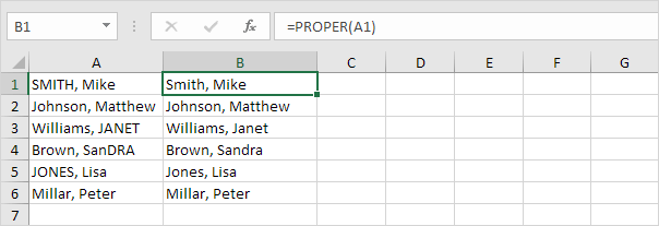
22. PROPER()
The PROPER() function capitalizes the first letter of each word in a text string.
‘=PROPER(A1)’ converts the text in this cell to the proper case or title case. Select and drag the cursor to apply it to other cells.
Logical formulas
23. IF()
The IF() function performs a logical test and returns one value if the condition is TRUE and another value if it is FALSE. It’s one of the most commonly used logical functions in Excel.
Formula: =IF(logical_test, value_if_true, value_if_false)
In this example, the formula in D2 checks if C2 is greater than B2. If true, it returns ‘Over Budget’; otherwise, it returns ‘Within Budget.’

24. IFERROR()
The IFERROR() function returns a specified value if a formula results in an error (like #DIV/0!, #N/A, etc.). If no error occurs, it returns the formula’s result.

25. ISERROR()
The ISERROR() function checks if a value results in any error and returns TRUE if it does or FALSE if it doesn’t. This function can be used to handle errors in formulas before they cause problems.

26. ISNUMBER()
The ISNUMBER() function checks if a value is a number and returns TRUE if it is, or FALSE if it isn’t. This is useful for validating data types in a range of cells.

Lookup functions and reference formulas
27. VLOOKUP()
VLOOKUP stands for ‘Vertical Lookup.’ It searches for a specific value in the first column of a table or range and returns a value in the same row from another column you specify. It is commonly used to retrieve data from a table based on a unique identifier.

28. HLOOKUP()
HLOOKUP stands for ‘Horizontal Lookup.’ It searches for a specific value in the top row of a table or range and returns a value in the same column from another row you specify. It is used similarly to VLOOKUP but works with data arranged horizontally.
The following example uses ‘=HLOOKUP(“March”, B1:G2, 2, FALSE)’.

29. INDEX()
The INDEX function returns the value of a cell in a specified row and column from within a given range. It is a versatile function often used in combination with other functions like MATCH.
This example uses ‘=INDEX(B2:D8,4,2)’.

30. INDEX-MATCH()
INDEX-MATCH is a powerful combination of two functions: INDEX and MATCH. It is used to perform more flexible lookups than VLOOKUP or HLOOKUP. The MATCH function finds the position of a value in a range, and INDEX returns the value at that position.
The formula used here in the example is: ‘=INDEX(B56:D63,MATCH(“Grapes”,A56:A63,0),2)

💡 Pro Tip: INDEX-MATCH is perfect for inventory management systems where you need to quickly look up data without manually searching through long lists.
32. INDIRECT()
INDIRECT returns a reference to a range or cell a text string specifies. This allows you to create dynamic references within your formulas.

Statistical formulas
33. MIN()
The MIN() function in Excel returns the smallest (minimum) value in a given range of numbers. This is useful when you need to identify the lowest value in a dataset.
For example, ‘MIN(number1, [number2], …)’. If it’s a range, then the formula will look something like, ‘=MIN(C2:C9)’

33. MAX()
MAX() is the opposite of MIN(). The MAX() function in Excel returns the largest (maximum) value in a range of numbers. This is useful for finding the highest value in a dataset.
For example, MAX(number1, [number2], …).

34. RANK()
The RANK() function in Excel returns a number’s rank in a list of numbers. The rank is based on its position in either ascending or descending order.
For example, RANK(number, ref, [order]).
- number: The number whose rank you want to find
- ref: The range of numbers you want to rank the number
- order: Optional. If 0 or omitted, ranks in descending order (from largest to smallest). If 1, ranks in ascending order (from smallest to largest)
35. PERCENTILE()
The PERCENTILE() function in Excel returns the value at a given percentile of a dataset. Percentiles are used to understand the distribution of data.
Formula: PERCENTILE(array, k)
- array: The range of values from which you want to find the percentile.
- k: The percentile value you want, between 0 and 1 (e.g., 0.25 for the 25th percentile).
In this example, the answer will be 1.5.

36. QUARTILE()
The QUARTILE() function in Excel returns the quartile of a dataset. Quartiles divide the data into four equal parts.
Formula: QUARTILE(array, quart)
- array: The range of values you want to find the quartile.
- quart: The quartile number you want to find (0 for the minimum value, 1 for the first quartile, 2 for the median, 3 for the third quartile, 4 for the maximum value).

Date and time formulas
37. NOW()
The NOW() function returns the current date and time based on your computer’s system clock. It updates every time the worksheet recalculates or when you open the workbook.
If you want to display the current date and time in a cell, simply use the NOW() function.

38. TODAY()
The TODAY() function returns the current date. Unlike NOW(), it does not include the time. It updates whenever the worksheet recalculates.
If today is September 02, 2025, and you want to display this date in a cell, the TODAY() function will return 02/09/2022.

39. EOMONTH()
The EOMONTH() function returns the last day of the month, which is a specified number of months before or after a given start date.
This is the syntax: ‘=EOMONTH(start_date, months)’

40. NETWORKDAYS()
The NETWORKDAYS() function calculates the working days (Monday to Friday) between two dates. It excludes weekends and, if provided, holidays.
Formula: =NETWORKDAYS(start_date, end_date, [holidays])

41. WORKDAY()
The WORKDAY() function returns a date that is a specified number of working days before or after a start date. It excludes weekends and can also exclude holidays if provided.
Formula: =WORKDAY(start_date, days, [holidays])

42. DAYS()
The DAYS() function returns the number of days between two dates. The formula is ‘=DAYS(end_date, start_date).’
For instance, to calculate the number of days between August 1, 2024, and August 31, 2024, you write, ‘=DAYS(‘8/31/2024’, ‘8/1/2024’),’ which will give you ‘30’.
Otherwise, if you find out today’s day, you can use ‘=DAY(TODAY()).’

43. DATEDIF()
The DATEDIF() function returns the difference between two dates in years, months, or days. This function is not documented in Excel but is helpful for date calculations.
Here’s the syntax: =DATEDIF(start_date, end_date, unit). The example uses ‘DATEDIF(A2, B2,’d’).

44. TIME()
The TIME() function converts hours, minutes, and seconds into a time format. It is helpful in constructing time values from individual components.
This is the formula you use, ‘=TIME(hour, minute, second).’

45. HOUR()
The HOUR() function extracts the hour from a time value. The syntax to use is ‘=HOUR(serial_number).’
If cell A1 contains the time ‘2:30:45 pm’, then your formula should be ‘=HOUR(A1).’ The answer would be 14.

46. MINUTE()
The MINUTE() function extracts the minutes from a time value. The syntax is ‘=MINUTE(serial_number)’.
If cell A1 contains the time 2:30:45 PM, then you would use ‘=MINUTE(A1)’. The answer would be ‘30’.

47. SECOND()
The SECOND() function extracts the seconds from a time value. In the example below, ‘=SECOND(NOW())’ is used.

Financial formulas
48. NPV()
The NPV() function calculates the Net Present Value of an investment based on a series of periodic cash flows (both incoming and outgoing) and a discount rate. In simpler terms, it helps determine if an investment will generate more than it costs. Thus, it’s widely used in financial analysis to give you a clearer picture of your potential returns.
For example, you are considering an investment that requires an initial outlay of $10,000 and is expected to generate returns of $3,000, $4,000, and $5,000 over the next three years.
If the discount rate is 10%, you can calculate the NPV as follows:
Formula: =NPV(0.10, -10000, 3000, 4000, 5000)
This would return an NPV of $782.59, which means the investment is expected to generate more value than its costs—always a good sign. If the NPV were negative, you’d know the project isn’t financially viable under the current assumptions.

49. IRR()
The IRR() function calculates the Internal Rate of Return for a series of cash flows.
The IRR is the discount rate that makes the NPV of the cash flows equal to zero. In other words, IRR tells you the rate of return that an investment is expected to generate over time.

Specialized formulas
50. SUBTOTAL()
The SUBTOTAL() function returns a subtotal in a list or database. It can perform various calculations, such as SUM, AVERAGE, COUNT, MAX, MIN, etc., on a range of data.
The main advantage of SUBTOTAL() is that it can ignore hidden rows, filtered data, or other SUBTOTAL() results within the range.

How to Use Formulas in Microsoft Excel
Getting the hang of Excel formulas can initially feel daunting, but once you get the basics down, you’ll wonder how you ever managed without them!
How do you use them? We’ll start with the basics and break it down step by step. Let’s suppose you want to calculate the profit from your sales and expenses units. We’ll show you how to insert formulas in Excel for this purpose.
Step 1: Enter your data
Before diving into formulas, make sure you input the data correctly. In this case, enter your sales figures and expenditure amounts in two separate columns.
For example, you could enter the sales data in column A and the expenses data in column B.

Bonus: How to Track Expenses in Excel!
Step 2: Select the cell for your formula
Next, choose the cell where you want the profit to be calculated. This is where your formula will be entered.
For example, if you want the profit to appear in column C, select the first cell in that column.

Step 3: Type the equal sign
In the selected cell, type in the equal sign ‘=’. This tells Excel that you’re entering a formula, not just plain text. It’s like a sign saying, “Here comes the math!”

Step 4: Enter the formula components
To calculate the profit, you need to subtract the expenditure amount in column B from the sales figure in column A.
After typing the equal sign, click on the first sales figure (e.g., A2). Then, type the minus sign ‘-’ to indicate subtraction. Click on the corresponding expenditure amount (e.g., B2). Your formula should look like this: =A2-B2.

Step 5: Press enter
After entering the formula in MS Excel, press the Enter key. Excel will automatically calculate the result and display the profit in the selected cell.
If you’ve done everything correctly, you should see the difference between your sales and expenditure amounts.

Step 6: Copy the formula down
To apply the same formula to other rows, simply click on the small square at the bottom-right corner of the cell containing your formula and drag it down to fill the range of cells in the column.
Excel will automatically adjust the cell references for each row, calculating the profit for each sales unit.

👀 Bonus: Integrate free spreadsheet templates into your workflow for increased efficiency and versatility.
Parts of an Excel Formula
A formula in Excel typically consists of any or all of the following:
- Functions
- Constants
- Operators
- References
Here is a simple example that will help you understand them properly.

The function PI() here returns the value of pi. The cell reference here is A2, which returns the value of cell A2.
At the same time, the constant is 2, referring to text or numeric values that are directly entered into the formula.
Lastly, the operator is the ^ (caret) that raises a number to a power. The formula also has * (asterisk), which is also an operator.
Functions
These are predetermined formulas that perform specific calculations. You can use them to perform simple or complex calculations.
To make things easier, Excel has an ‘Insert Function’ dialog box to help you add functions to your formula.
Constants
A constant in a formula is a fixed value that cannot be calculated; it remains the same.
For example, the number 450, the date 12/06/2020, or even text such as ‘Expenditure’ are called constants.
Operators
Operators in Excel are symbols that specify the type of calculation or comparison in a formula. They help you manipulate and analyze data efficiently.
There are various types of operators that you can use for different purposes:
- Arithmetic: The minus, plus, asterisk, and percent signs all fall under this kind of operator
- Comparison: The equal, greater than, less than, and other such signs help you compare two values
- Text concatenation: This type of operator uses the ampersand (&) to join one or more text strings and produce one text string. For example, ‘South’ & ‘West’ becomes ‘Southwest’
References
References in Excel are cell addresses used in formulas to point to specific data points. They are essential for creating dynamic and flexible formulas that automatically adjust when data changes.
These allow formulas to interact dynamically with your spreadsheet’s values and data.
The Benefits of Using Formulas in Excel
Excel’s fundamental advantage lies in its extraordinary data organization features. However, a simple grid serves no complex function except storing your data in an organized way, until you deploy the software’s formulas.
Excel formulas can speed up and improve your work, whether you’re crunching numbers, analyzing data, or simply keeping things organized.
Now that you know Excel formulas help data analysis, let’s look into their benefits:
Increasing efficiency
Excel formulas automate repetitive calculations.
Ever spent hours adding up numbers or performing repetitive calculations? With Excel formulas, those tasks are a breeze. For example, you can instantly apply the ‘SUM’ function to hundreds of datasets.
This reduces the painstaking manual data entry process, while speeding up your work and minimizing the chance of errors.
Gaining valuable insights
Excel formulas let you dive deeper into your data.
For instance, with pivot tables, you can apply conditional formatting and group dates for better analysis. You can also add date timelines, sort and rank columns, and run total checks on large datasets.
This Excel function makes it easier to analyze and understand your data.
Performing conditional analysis
Do you need to make decisions based on specific conditions? Excel’s IF and SUMIF functions can help. These functions allow you to perform calculations based on specific conditions, enabling you to predict outcomes and compare different datasets.
With these formulas, you can set up criteria to evaluate scenarios, helping you make data-backed decisions.
Facilitating financial planning
Many companies use formulas in Excel for financial modeling. Functions such as NVP (Net Present Value) and IRR (Internal Rate of Return) help users evaluate investment opportunities.
Meanwhile, formulas like ‘SUMIFs’ and ‘FORECAST’ create detailed forecasts that support planning. These functions help you streamline your business operations.
Enhancing versatility
Excel’s versatility is one of the main reasons it’s so widely used across different industries.
You’ll often see Excel proficiency listed as a must-have skill in job descriptions for fields like finance, marketing, data science, and more. That’s because Excel can tackle everything from basic formulas and calculations to complex data analysis.
Excel’s versatility makes it a must-have skill for budgeting, analyzing data, and forecasting trends.
Limitations of Using Excel Formulas
Excel formulas aren’t without their downsides. While Excel is widely used and accessible, relying on it for complex tasks can lead to errors and limitations that may hinder your workflow.
Here are some reasons why Excel might not always be the best choice.
Complex nested formulas
When you’re working with complicated problems, Excel formulas can quickly become overwhelming.
Writing long nested formulas isn’t just difficult; it’s also easy to make mistakes that are hard to catch. A single misstep in your formula can throw off your entire calculation.
If your requirements change, you’ll have to edit those formulas again, which can be tedious.
And if someone else picks up your workbook? It’s difficult to understand the original logic, and this is a common frustration many teams face with complicated data sets.
Difficult to maintain
Maintaining and documenting Excel formulas is challenging, especially when dealing with complex problems.
With multiple contributors, edits, and updates, keeping your spreadsheet organized becomes more daunting over time.
Performance issues with large datasets
As your datasets grow, Excel’s performance slows down. Aggregating thousands of rows of data can make even the simplest calculation a major time sink.
Aggregating and synthesizing large tables can become overwhelming, leading to slow calculations and making navigating and interpreting your data hard. This performance hit is one of the critical limitations of relying heavily on Excel for large-scale data analysis.
Suddenly, you’re waiting for formulas to recalculate, scrolling through endless rows and hoping your spreadsheet doesn’t crash.
Sound familiar? That’s because Excel isn’t optimized for handling massive datasets.
Integration challenges with other software
While Excel integrates well with other Microsoft Office apps like Word and PowerPoint, it doesn’t play as nicely with other software. This limited integration can make transferring data from Excel to other tools tedious.
Exporting data into other systems often requires extensive manual adjustments, which can break your workflow and consume time.
This lack of seamless integration can be a major headache when you’re using Excel alongside specialized software or other project management tools.
Wouldn’t it be nice if everything just…worked together?
Lack of collaboration capabilities
Collaborating on Excel files isn’t always as smooth as you’d like.
Between version control issues, broken links, and permission errors, teamwork can quickly get derailed. These issues can slow down collaboration and introduce risks that other tools might not present. Unlike modern tools that offer real-time collaboration, Excel makes it easy to end up with conflicting versions of the same file. Not exactly teamwork-friendly, right?
That’s why it’s worth considering Excel alternatives that might better suit your needs for more advanced or collaborative tasks.
Meet ClickUp: The Best Excel Alternative
It’s time for an alternative—something more intuitive, flexible, and designed for modern workflows. Enter ClickUp, an innovative Excel alternative designed to make your life easier.
ClickUp provides an efficient way to manage your tasks and projects, tackling issues like complex formulas and slow performance.
See how ClickUp can be the breakthrough you need for a more organized and productive workflow. ⬇️
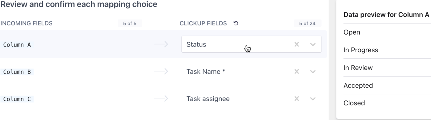
💡 Pro Tip: ClickUp’s Spreadsheet Importer makes it super simple to import and map your data from Excel, CSV, XML, JSON, TSV, or TXT files! Try it today.
ClickUp’s Table View
ClickUp’s Table View provides a versatile, spreadsheet-like format that helps you easily organize and manage tasks.
It allows you to structure your data effectively, with each row representing a task and each column capturing various attributes such as progress, file attachments, or ratings.

ClickUp Custom Fields allow you to tailor the workspace to fit your specific needs.
With support for over 15 different field types, you can capture and display a wide range of data relevant to your projects.
Bulk editing further simplifies your workflow by letting you update multiple tasks at once, saving you from the repetitive task of editing each entry individually. Additionally, exporting your data as CSV or Excel files is straightforward, ensuring you can easily share or analyze it.

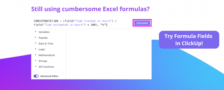
ClickUp Formula Fields
ClickUp Formula Fields offers a powerful way to perform complex calculations directly within your tasks.
Setting up a Formula Field is simple: click the ➕ icon icon above your task table, choose Formula, and give it a name. 🎯.
You can use basic mathematical operations for quick calculations or the Advanced Editor for more complex formulas.

💡 Pro Tip: Pin a column to keep it visible as you scroll through your Table. Just click the column title you want to pin and select ‘Pin Column.’ This way, important information stays in view as you navigate your data.
Simple Formulas handle basic arithmetic like addition or subtraction, which is useful for straightforward calculations such as finding the difference between costs and revenues.
Advanced Formulas, on the other hand, support a variety of functions and more intricate calculations. You can use functions like IF, DAYS, and ROUND to create formulas that handle complex logic, such as calculating the time remaining or assessing task deadlines.
Other advanced formulas for various use cases include:
- Date and time functions
- String functions
- Mathematical functions
Automation capabilities
ClickUp’s Automation capabilities integrate seamlessly with Formula Fields in Table View. This allows you to set up automation based on dynamic data, helping you streamline repetitive tasks and improve efficiency.
For example, you can create an automation that triggers an alert when specific conditions in your formulas are met, helping you stay on top of important tasks and updates.
Beyond data organization and calculation, ClickUp offers several other features to enhance your workflow. You can share your Table View with others through publicly shareable links, making it easy to keep clients or team members informed.

You can also copy-paste information into other spreadsheet software for easier accessibility.
ClickUp allows you to format tables, filter and group information, and hide columns to manage your data better. You can also drag and drop columns for easy reorganization, ensuring your Table View adapts to your needs.

👀 Bonus: Spreadsheets don’t usually have built-in alert systems, which can lead to missed deadlines. Set up project management automation in ClickUp to notify team members of upcoming deadlines, overdue tasks, or important updates.
From Excel Limitations to ClickUp Solutions
Microsoft Excel is an excellent tool for professionals in various industries, and Excel formulas remain its backbone. However, it comes with its own set of limitations. From the challenge of maintaining complex nested formulas to performance issues with large datasets, Excel can sometimes fall short.
This is where having an alternative like ClickUp comes in handy.
ClickUp helps organize large datasets that otherwise cause information overload. The quick and easy-to-use software enables seamless collaboration with team members.
Bringing its advanced formulas to the ‘table’ (pun intended), ClickUp is a powerful tool for flexible data management solutions.
Sign up to ClickUp and experience its impact on your data management today! 🚀

Everything you need to stay organized and get work done.