How to Calculate Time in Excel (A Complete Tutorial and Helpful Formulas)

If you’ve been relying on Excel to manage your projects and need help with time calculations, you’re not alone. Figuring out the elapsed time of a project or task is crucial for team leads who need to know what work should be prioritized and how to properly allocate resources.

Simply put, time values are tricky in Excel—especially when calculating time difference, hours worked, or the difference between two employees.

Luckily for you, we’ve done all the hard work to help format cells and calculate elapsed time in Excel faster. Let’s get confident about using Excel for project time tracking and discover the various ways of tracking time.

What Types of Time Calculations Can You Perform in Microsoft Excel?

There isn’t a single formula or format for calculating time in Excel. It depends on your dataset and the goal you want to achieve. Most use a custom format (number over text function) to display time and date values or time differences.

But there are two types of calculations to get you started, which include:

1. Add time: If you need to obtain the sum of two time values to get a total
   • Add up to less than 24 hours: When you need to know how many hours and minutes it’ll take to complete two simple tasks
   • Add up to more than 24 hours: When you need to add the estimated or actual elapsed time of multiple slow, complex tasks
2. Subtract time: If you need to get the total time between a start and an end time
   • Subtract times whose difference is less than 24 hours: When you need to figure out the hours elapsed since a team member started to execute a simple task
   • Subtract times whose difference is more than 24 hours: When you need to know the hours that have gone by since your project started

How Do You Calculate Time and Hours in Excel Using Formulas and Cell Formatting?

Time calculations in Excel work by subtracting or adding time-formatted numeric values. You enter start and end times in cells, apply subtraction or SUM formulas, and then convert the result using Custom or Number formatting. Without proper formatting, Excel displays incorrect values. Both elapsed time and total working hours rely on numeric date-time conversion.

Let’s go through a few formulas for time calculations in Excel, so you get down to the exact hours, minutes, and seconds in your custom time format.

Time Difference in Excel

Before we teach you how to calculate time in Excel, you must understand what time values are in the first place. Time values are the decimal numbers to which Excel applied a time format to make them look like times (i.e., the hours, minutes, and seconds).

Because Excel times are numbers, you can add and subtract them. The difference between a start time and an end time is called the “time difference” or “elapsed time.”

These are the steps to subtract times whose difference is less than 24 hours:

1. Enter the start date and time in cell A2 and hit Enter. Don’t forget to write “AM” or “PM”
2. Enter the end time in cell B2 and hit Enter
3. Enter the formula =B2-A2 in cell C2 and hit Enter.

^WARNING
As you can tell from the figure, this formula doesn’t work for times that belong to different days. This example shows the time difference between two time values within a 24-hour time period.

4. Right-click on C2 and select Format Cells.

5. Choose the Custom category and type “h:mm”

^{SIDE NOTE}
You might wish to obtain the time difference expressed in hours or hours, minutes, and seconds. If so, type “h” or “h:mm:ss,” respectively. This will help you avoid negative time values.

6. Click OK to see the total change to a format describing only the number of hours and minutes in the elapsed time between A2 and B2.

Check out our detailed blog to find a list of time management strategies you can use right away!

Date and time in Excel

In the previous section, you learned how to calculate hours in Excel. But the formula you learned only applied to time differences of less than 24 hours.

If you need to subtract times whose difference is more than 24 hours, you need to work with dates instead of times. Do it like this (format cells dialog box):

1. Enter the start time in cell A2 and hit Enter.
2. Enter the end time in cell B2 and hit Enter.
3. Right-click on A2 and select Format Cells.
4. Choose the Custom category and type “m/d/yyyy h:mm AM/PM.”
5. Click OK to see A2 change to a format starting with “1/0/1900” and adjust the date.
6. Use the Format Painter to copy the formatting of A2 to B2 and adjust the date.
7. Enter the formula =(B2-A2)*24 in cell C2 and hit Enter to see the total change to a format describing the number of hours in the time elapsed between A2 and B2.

^WARNING
You must apply the “Number” format to C2 to get the correct value in the above formula.

Sum time in Excel

Suppose you want to sum up the time difference between your team members working on multiple project tasks. If those durations add up to less than 24 hours, follow these steps:

1. Enter one duration in cell B2 (with the format h:mm) and hit Enter.
2. Enter the other duration in cell B3 and hit Enter.
3. Enter the formula =B2+B3 in cell B4 and hit Enter.

^{PRO TIP}
If you prefer clicking a single button instead of entering a formula, you may position the cursor in B4 and hit the Σ (or AutoSum) button in the Home tab. The button will apply the formula =SUM(B2:B3) to the cell in the above example.

If the total duration of your project tasks adds up to more than 24 hours, follow these steps instead:

1. Enter one duration in cell B2 (with the format h:mm) and hit Enter. (Warning: Beware that the maximum duration is 23 hours and 59 minutes)
2. Enter the other duration in cell B3 and hit Enter.
3. Enter the formula =B2+B3 in cell B4 and hit Enter.
4. Right-click on B4 and select Format Cells.
5. Choose the Custom category and type “[h]:mm;@.”
6. Click OK to see B4 correctly displaying the sum of the times in B2 and B3.

If you’d like to know more about Excel project management, our blog is the perfect place to start!

More Excel Resources:

• Create a timeline in Excel
• Create a dashboard in Excel
• Create a calendar in Excel
• Create an org chart in Excel
• Create a schedule in Excel
• Capacity planning in Excel

What Are the Most Useful Excel Formulas for Time Calculations?

Excel offers dedicated formulas for calculating hours, minutes, seconds, and elapsed time using subtraction, TIMEVALUE, TEXT, INT, NOW, and arithmetic multipliers. Results depend heavily on cell formatting and whether differences exceed 24 hours. Some formulas return numeric values, while others output text for reporting. Incorrect formatting is the main cause of calculation errors.

It pays to know the formulas when you’re calculating time differences in Excel. To get your time difference and value set up correctly, we’ve provided a list of formulas to make your calculations easier.

Formula	Description
=B2-A2	Difference between the two time values in cells A2 and B2
=(B2-A2)*24	Hours between the value in cells A2 and B2 (24 being the number of hours in a day)   Warning: If the difference is 24+ hours, you must apply the “Custom” format with the type “m/d/yyyy h:mm AM/PM” to A2 and B2. You also must apply the “Number” format to the cell containing the time difference formula.
=TIMEVALUE(“8:02 PM”)-TIMEVALUE(“9:15 AM”)	Warning: The difference must be less than 24 hours.
=TEXT(B2-A2,”h”)	Hours between the values in cells A2 and B2   Warning: You must apply the “Custom” format with the type “h” to A2 and B2. Also, the value in B2 cannot be less than A2 and the difference must be less than 24 hours to avoid a negative value. And the TEXT function returns a textual value.
=TEXT(B2-A2,”h:mm”)	Minutes and hours between the time values in cells A2 and B2.   Warning: You must apply the “Custom” format with the type “h:mm” to A2 and B2. Also, the value in B2 cannot be less than A2 and the difference must be less than 24 hours.
=TEXT(B2-A2,”h:mm:ss”)	Hours, minutes, and seconds between the time values in cells A2 and B2.   Warning: You must apply the “Custom” format with the type “h:mm:ss” to A2 and B2. And the value in B2 cannot be less than A2 and the difference must be less than 24 hours.
=INT((B2-A2)*24)	Number of complete hours between the time values in cells A2 and B2 (24 being hours in a day).   Warning: If the difference is 24+ hours, you must apply the “Custom” format with the type “m/d/yyyy h:mm AM/PM” to A2 and B2. And you must apply the “Number” format to the cell containing the time difference formula.
=(B2-A2)*1440	Minutes between the time values in cells A2 and B2 (1440 being minutes in a day). Warning: If the difference is 24+ hours, you must apply the “Custom” format with the type “m/d/yyyy h:mm AM/PM” to A2 and B2. And you must apply the “Number” format to the cell containing the time difference formula.
=(B2-A2)*86400	Seconds between the time values in cells A2 and B2 (86400 being the seconds in a day).   Warning: If the difference is 24+ hours, you must apply the “Custom” format with the type “m/d/yyyy h:mm AM/PM” to A2 and B2. And you must apply the “Number” format to the cell containing the time difference formula.
=HOUR(B2-A2)	Hours between the time values in cells A2 and B2. Warning: The value in B2 cannot be less than the value in A2 and the difference must be less than 24 hours. Also, the HOUR function returns a numeric value.
=MINUTE(B2-A2)	Minutes between the time values in cells A2 and B2.   Warning: The value in B2 cannot be less than the value in A2 and the difference must be less than 60 minutes. Also, the MINUTE function returns a numeric value.
=SECOND(B2-A2)	Seconds between the time values in cells A2 and B2.   Warning: The value in B2 cannot be less than the value in A2 and the difference must be less than 60 seconds. Also, the SECOND function returns a numeric value.
=NOW()-A2	Time elapsed between the date and time in cell A2 and the current date and time.   Warning: If the elapsed time is 24+ hours, you must apply the “Custom” format with the type “d “days” h:mm:ss” to the cell containing the time difference formula. Also, Excel doesn’t update the elapsed time in real-time. To do that, you must hit Shift+F9.
=TIME(HOUR(NOW()),MINUTE(NOW()),SECOND(NOW()))-A2	Time elapsed between the value in cell A2 and the current date and time.   Warning: Excel doesn’t update the elapsed time in real-time. To do that, you must hit Shift+F9.
=INT(B2-A2)&” days, “&HOUR(B2-A2)&” hours, “&MINUTE(B2-A2)&” minutes, and “&SECOND(B2-A2)&” seconds”	Time elapsed between the date and time or time values in cells A2 and B2, expressed in the format “dd days, hh hours, mm minutes, and ss seconds.”   Warning: This formula returns a textual value. If you need the result to be a value, use the formula =B2-A2 and apply the “Custom” format with the type “d “days,” h “hours,” m “minutes, and” s “seconds”” to the cell containing the time difference formula.
=IF(INT(B2-A2)>0,INT(B2-A2)&” days,”,””)&IF(HOUR(B2-A2)>0,HOUR(B2-A2)&” hours,”,””)&IF(MINUTE(B2-A2)>0,MINUTE(B2-A2)&” minutes, and “,””)&IF(SECOND(B2-A2)>0,SECOND(B2-A2)&” seconds”,””)	Time elapsed between the date and time or values in cells A2 and B2, expressed in the format “dd days, hh hours, mm minutes, and ss seconds” with zero values hidden.   Warning: This formula returns a textual value. If you need the result to be a value, use the formula =B2-A2 and apply the “Custom” format with the type “d “days,” h “hours,” m “minutes, and” s “seconds”” to the cell containing the time difference formula.
=A2+TIME(1,0,0)	Value in cell A2 plus one hour.   Warning: This formula only allows adding less than 24 hours to a value.
=A2+(30/24)	Value in cell A2 plus 30 hours (24 being hours in a day).   Warning: This formula allows adding any number of hours to a value.
=A2-TIME(1,0,0)	Time value in cell A2 minus one hour.   Warning: This formula only allows subtracting less than 24 hours from a value.
=A2-(30/24)	Time value in cell A2 minus 30 hours.   Warning: This formula allows subtracting any number of hours from a value.
=A2+TIME(0,1,0)	Time value in cell A2 plus one minute.   Warning: This formula only allows adding less than 60 minutes to a value.
=A2+(100/1440)	Time value in cell A2 plus 100 minutes (1440 being minutes in a day).   Warning: This formula allows adding any number of minutes to a value.
=A2-TIME(0,1,0)	Time value in cell A2 minus one minute.   Warning: This formula only allows subtracting less than 60 minutes from a value.
=A2-(100/1440)	Time value in cell A2 minus 100 minutes.   Warning: This formula allows subtracting any number of minutes from a value.
=A2+TIME(0,0,1)	Time value in cell A2 plus one second.   Warning: This formula only allows adding less than 60 seconds to a value.
=A2+(100/86400)	Time value in cell A2 plus 100 seconds (86400 being seconds in a day). Warning: This formula allows adding any number of seconds to a value.
=A2-TIME(0,0,1)	Time value in cell A2 minus one second.   Warning: This formula only allows subtracting less than 60 seconds from a value.
=A2-(100/86400)	Time value in cell A2 minus 100 seconds.   Warning: This formula allows subtracting any number of seconds from a value.
=A2+B2 =SUM(A2:B2)	Total hours, hours and minutes, or hours, minutes, and seconds in the values from cells A2 and B2, depending on the format you applied to those cells.   Warning: If the total adds up to more than 24 hours, you must apply the “Custom” format with the type “[h]:mm;@” to the cell containing the SUM formula.

🎥 See how this small business moved away from a sheet-based workflow!

What Is an Easier Alternative to Manual Time Calculations in Excel?

Although the formulas in this article work, there’s a better way than Excel to calculate time—ClickUp!

Instead of building and maintaining complex formulas, you can track time directly using built-in date and time fields inside ClickUp’s Converged AI workspace.

Here’s what that looks like in practice:

Track time without leaving your tasks

ClickUp has a built-in global timer that works across the web, desktop, and mobile apps. Start a timer on your laptop, stop it from your phone. No Chrome extension required.

You can also manually add time entries by typing natural durations like “2h 30m” or “2:30” directly from Table View, List View, Board View, Gantt View, or the floating toolbar. Every entry can be tagged as billable or non-billable, labeled with custom tags, and annotated with descriptions.

Calculate time automatically with Formula Fields

This is where ClickUp replaces Excel’s time formulas entirely.  Formula Fields support 70+ functions and can reference:

• Time Tracked and Time Estimated (in hours)
• Start Date, Due Date, Date Created, Date Closed, Date Updated
• Sprint Points, Number fields, Currency fields, and other Formula Fields

For example, you can calculate the cost of work with field("Hourly Rate") * field("Time Tracked"), or find the project duration with DAYS(field("Due Date"), field("Start Date")). ClickUp’s date and time functions include DAYS, MONTH, YEAR, NETWORKDAYS, WEEKDAY, EDATE, EOMONTH, and more. You can even ask ClickUp AI to write formulas for you.

Get instant totals with column calculations

No SUM formula needed. In Table View or List View, hover over any column and click Calculate to see:

• Sum, Average, Median, Min, Max, Range for numeric and time fields
• Earliest date, Latest date, Date range for date fields
• Count, Count unique, Percent empty/not empty for any field

Time tracked on subtasks automatically rolls up to parent tasks, and column calculations include those rolled-up values. Group your Table View by assignee or status, and you’ll see calculations per group plus a total across the entire view.

This simple interface lets you drag and drop rows and columns to quickly change your view.

Manage timesheets and approvals in one place

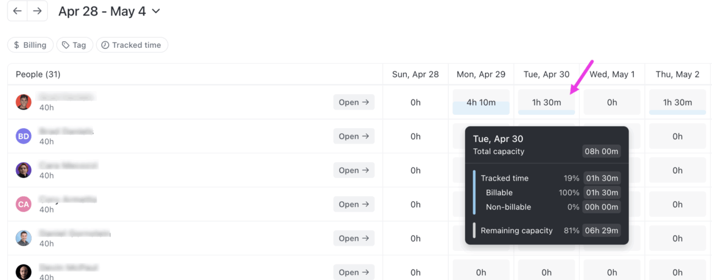
The Timesheets Hub gives you a dedicated space to view all tracked time by task or by date. Set your weekly capacity, filter by billable or non-billable entries, and add time tracking labels to categorize your hours.

You can also use Timesheet Approvals to run a full submit, review, and approve workflow. Team members submit their weekly timesheets, managers approve or request changes, and time entries lock upon submission, so nothing gets accidentally modified. You can even bulk-approve multiple timesheets at once.

Plan your time with AI

Forget manually planning time. These three features take care of it all:

• The Calendar in ClickUp uses AI to automatically time-block your top-priority tasks. Drag tasks into the schedule and let AI handle the rest.
• The Teams Hub gives managers a bird’s-eye view of team timesheets, activity, and capacity from a single screen
• Super Agents, ClickUp’s AI-powered teammates, can generate billable hours summaries, analyze workload capacity, and flag projects that are over budget, all on a schedule you set

Visualize time data on Dashboards

Build Dashboards with Timesheet cards, Calculation cards (sum, average, min, max), and Bar or Pie charts grouped by time tracked, assignee, or status. AI Dashboard templates like the AI Team Center give you pre-built views of your team’s time and productivity data with zero setup.

Track and evaluate idle time using the ClickUp Time Analysis Template

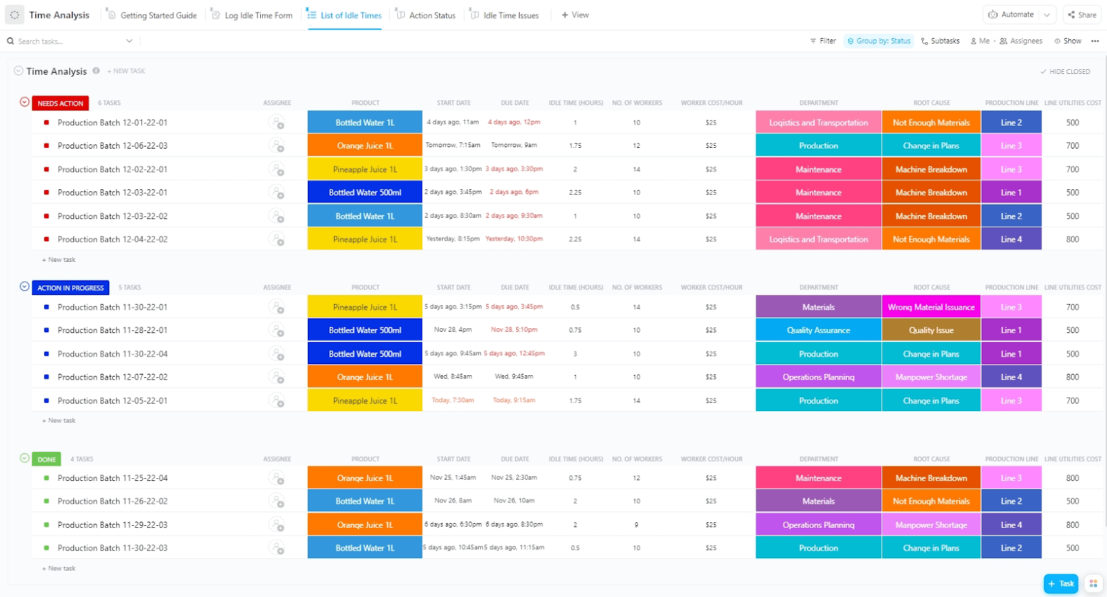
If you don’t want to start from scratch, try ClickUp’s Time Analysis Template to get started! This template allows you to monitor project timelines, track individual task times, and analyze time spent on each task or project for comprehensive oversight.

By providing a clear, comprehensive view of time utilization, it helps drive productivity and ensure efficient resource allocation. Say goodbye to complicated Excel formulas and start optimizing your team’s time management with ClickUp!

Want to retain your spreadsheets in Excel or Google Sheets, but have the ability to do more, faster with your data? Try the Spreadsheet Template by ClickUp. It helps you:

• Organize spreadsheets into one centralized system
• Track changes over time and collaborate with teammates
• Access and update your data from anywhere in the world with ease
• Integrate data with other ClickUp tools, such as Chat and Docs

Don’t believe us? Try ClickUp today and make spreadsheet chaos a thing of the past!

Explore article topics