7 Best VLOOKUP Alternatives (Better Lookup Functions)

Say you’re working on a product launch and have compiled the customer information, order details, supplier contacts, task owners, and timelines across different tabs and spreadsheets. 

VLOOKUP formulas fetch customer details from one sheet, match them with product orders in another, and calculate expected delivery dates for you. But here’s the catch: now you have to add an additional column, and you’re worried the compiled data will fall apart. 

To avoid this, you can either turn to more flexible VLOOKUP alternatives or abandon traditional spreadsheets and use ClickUp, an all-in-one workflow management software.

Let’s check it out together. 

Summarize this article with AI ClickUp Brain not only saves you precious time by instantly summarizing articles, it also leverages AI to connect your tasks, docs, people, and more, streamlining your workflow like never before. Summarize article

Summarize this article for me please

Want to save even more time? Try ClickUp Brain free

What Is VLOOKUP and Why Look for Alternatives?

VLOOKUP, short for ‘Vertical Lookup,’ is an Excel function designed to search for a specific value in the first column of a table and return a corresponding value from another column in the same row.

It’s commonly used for tasks like matching product IDs to prices or retrieving an employee code based on their names.

Summarize this article with AI ClickUp Brain not only saves you precious time by instantly summarizing articles, it also leverages AI to connect your tasks, docs, people, and more, streamlining your workflow like never before. Summarize article

Summarize this article for me please

Want to save even more time? Try ClickUp Brain free

⭐️ Featured Template

The ClickUp Spreadsheet Template offers a flexible way to organize, filter, and analyze data—making it a powerful alternative to traditional VLOOKUP functions. With built-in collaboration and automation features, it streamlines complex data management without the need for advanced formulas.

Get free template

Common use cases for VLOOKUP

Wondering when you should use VLOOKUP? Here are the most common use cases where you can quickly connect information across table templates:

• Fetch related data from a lookup table. For instance, you can look up an employee’s ID to find their name or department
• Compare two columns to identify common entries or differences, like determining which customers in one list also appear in another
• Pull data from one worksheet into another, consolidating information spread across multiple sheets
• Cross-reference entries against a master list with VLOOKUP to validate data and ensure consistency and accuracy across datasets

Limitations of VLOOKUP

While the VLOOKUP formula works as a one-function tool for basic, table-based lookups, its simplicity has some critical drawbacks. Here are a few of them:

• Rigid column structure: VLOOKUP requires the lookup column to be the leftmost in the table array, as it cannot search to the left, limiting flexibility in data organization
• Fragile to structural changes: Inserting or deleting columns within the table can break the function, as it relies on fixed columns
• Performance issues: It can slow down performance in large datasets, especially when used extensively across numerous rows
• Limited to single matches: VLOOKUP returns only the first match it finds, which can be problematic if multiple entries share the same lookup value
• Error-prone: If the lookup value isn’t found, VLOOKUP returns a #N/A error, which can disrupt data analysis if not handled properly

Summarize this article with AI ClickUp Brain not only saves you precious time by instantly summarizing articles, it also leverages AI to connect your tasks, docs, people, and more, streamlining your workflow like never before. Summarize article

Summarize this article for me please

Want to save even more time? Try ClickUp Brain free

Top VLOOKUP Alternatives in Excel and Google Sheets

Excel offers many replacements for VLOOKUP for everyone who wants to simplify their data management process. Here are a few of them!

1. INDEX and MATCH functions

The INDEX MATCH function is a solid replacement for VLOOKUP due to its flexibility and precision. Unlike VLOOKUP, which can only search from the leftmost column to the right, INDEX MATCH allows you to perform lookups in any direction—left, right, up, or down.

The MATCH function locates a lookup value’s position or row number in a range, while the INDEX function returns the value at that position in a separate range. 

This decoupling of lookup and return columns makes the formula less rigid; you can insert or delete columns without breaking them. 

Let’s find the ID of ‘Kathleen Hanner’ using the ‘full name column’ (Column I). 

The formula mentioned is: =INDEX(return_range, MATCH(lookup_value, lookup_range, 0))

This is what the Index Match functions mean here:

• return_range: The range containing the values you want to return (e.g., H2:H10)
• lookup_value: The value you are searching for (e.g., “Kathleen Hanner”)
• lookup_range: The range where you want to search for the lookup_value (e.g., I2:I10)
• 0: Specifies an exact match in the MATCH function

Hence, the final formula for the INDEX MATCH combination: =INDEX(H2:H10, MATCH(“Kathleen Hanner”, I2:I10, 0))

✅ Final output: 3549

2. XLOOKUP (Excel only)

While the INDEX MATCH formula splits the task across two functions, the Excel XLOOKUP function combines lookup and return logic into a more intuitive formula. It is Excel’s modern answer to VLOOKUP’s limitations and works seamlessly across well-structured source data.

It requires three main inputs: the lookup value, the lookup array (where to search), and the return array (what to return once found), to search lookups in every direction.

XLOOKUP also handles exact matches by default, supports search modes (e.g., reverse search), and returns custom values when no match is found, eliminating the need for IFERROR.

Let’s focus on the ID of ‘Earlean Melgar’ in column I:

The formula mentioned is: =XLOOKUP(lookup_value, lookup_range, return_range)

Check out this breakdown of the Excel XLOOKUP function:

• lookup_value: The value you’re searching for (e.g., “Earlean Melgar”)
• lookup_range: The column or row to search in (e.g., I2:I10)
• return_range: The range to return a value from (e.g., H2:H10)

Hence, the formula: =XLOOKUP(“Earlean Melgar”, I2:I10, H2:H10)

✅ Final output: 2456

📌Unlike MATCH, XLOOKUP performs an exact match by default, so you don’t need to specify 0.

3. FILTER function (Google Sheets)

The FILTER function is a Google Sheets-only alternative that returns all matching values, not just the first one. It auto-pulls rows or columns based on conditions you define, making it ideal for extracting entire datasets that meet specific criteria, something the VLOOKUP function can’t do without an array formula or helper column. 

FILTER is also array-native, meaning it automatically spills results without needing Ctrl+Shift+Enter. It suits dashboards, reports, or flexible, multi-row lookups.

Let Google Sheets scan column H to find out the employee’s name with ID 2587!

The formula mentioned is: =FILTER(return_range, condition_range = lookup_value)

This is the breakdown: 

• return_range: The values you want to extract (e.g., I2:I10)
• condition_range: The range where the condition is applied (e.g., H2:H10)
• Lookup_value: The value you’re checking against (e.g., 2587)

Hence, the Google Sheets formula: =FILTER(I2:I10, H2:H10 = 2587)

✅ Final output: Philip Gent

4. QUERY function (Google Sheets)

QUERY turns your spreadsheet into a database by allowing you to use SQL-like commands (e.g., SELECT, WHERE, ORDER BY) directly on your data. It’s more readable for complex lookups and data manipulations, such as returning multiple rows that meet a bunch of conditions. 

Unlike VLOOKUP, QUERY doesn’t require your lookup column to be in the first position. It references columns by label or position in any order. It’s especially useful for reporting, filtering, grouping, or summarizing data without writing multiple nested formulas.

Here, Google Sheets reads the formula as ‘From the range A1 to I10, return the value in column I where column B has the value ‘Earlean’’.

The formula mentioned is: =QUERY(data_range, “SELECT return_column WHERE condition_column = ‘lookup_value'”, headers)

Here’s the breakdown:

• data_range: The full table or dataset to query (e.g., A1:I10)
• return_column: The column you want to return data from (e.g., column I)
• condition_column: The column to apply the condition on (e.g., column B)
• lookup_value: The number of header rows in the data (e.g., 1)

Hence, the formula: =QUERY(A1:I10, “SELECT I WHERE B = ‘Earlean'”, 1)

✅ Final output: Earlean Melgar

📌 This QUERY formula is SQL-style and returns values from column I where column B equals ‘Earlean’.

5. LOOKUP formulas

The LOOKUP function searches vertically and horizontally, but only when the lookup range is sorted in ascending order. When working across different data shapes, it’s more forgiving than the VLOOKUP function because it doesn’t restrict you to left-to-right lookups. 

However, its reliance on sorted data and lack of error handling make it less practical in modern workflows. Still, it can be handy for quick, approximate matches or when working with legacy files where other functions aren’t available.

Excel scans down column H, finds the closest match ≤ 2587, and returns the corresponding name from column I. 

The formula mentioned is: =LOOKUP(lookup_value, lookup_range, return_range)

Here’s the breakdown:

• lookup_value: The value you’re searching for (e.g., 2587)
• lookup_range: The range where the value is searched (e.g., H2:H10)
• return_range: The range to return a corresponding value from (e.g., I2:I10)

Hence, the formula: =LOOKUP(2587, H2:H10, I2:I10)

✅ Final output: Gaston Brumm

6. OFFSET + MATCH FUNCTION

The OFFSET + MATCH combination offers lookups by returning a cell reference based on a starting point, row/column offsets, and a match condition. It’s useful when your lookup values don’t fall into a fixed structure or your data range shifts over time. 

MATCH locates the relative position, and OFFSET uses that to find the return cell. This formula is highly flexible for dynamic ranges, shifting data tables, or extracting values based on variable positions.

Let’s find out the age of Philip Gent in the data below!

The formula mentioned is: =OFFSET(reference_cell, MATCH(lookup_value, lookup_range, 0), column_offset)

Here’s how the breakdown would look: 

• reference_cell: The starting cell for OFFSET (e.g., G1)
• lookup_value: The value you’re trying to match (e.g., “Philip Gent”)
• lookup_range: The range where the lookup is performed (e.g., I2:I10)
• column_offset: The number of columns to offset from the starting cell (e.g., 0 means stay in the same column)

Hence, the formula: =OFFSET(G1, MATCH(“Philip Gent”, I2:I10, 0), 0)

✅ Final output: 36

7. Indirect-Address-Match 

This trio leverages INDIRECT and ADDRESS to build cell references, and MATCH finds the target row or column. It’s particularly useful when the worksheet or cell reference needs to change based on input values, something VLOOKUP can’t handle. 

For example, you can build formulas that look up data across multiple sheets or change table structures. However, INDIRECT is volatile, meaning it recalculates frequently and may slow down large files.

Let’s find the age of Vincenza Weiland!

The formula mentioned is: =INDIRECT(ADDRESS(MATCH(lookup_value, lookup_range, 0) + row_offset, column_number))

• lookup_value: The value you’re trying to find (e.g., “Vincenza Weiland”)
• lookup_range: The range where the lookup is performed (e.g., I2:I10)
• row_offset: The number added to the MATCH result to adjust the final row (e.g., + 1)
• column_number: The numeric column index to return from (e.g., 7 = column G)
• ADDRESS: Constructs the cell reference based on row and column numbers
• INDIRECT: Converts that reference into a value by pointing to the actual cell

Hence, the formula:  =INDIRECT(ADDRESS(MATCH(“Vincenza Weiland”, I2:I10, 0) + 1, 7))

✅ Final output: 40

Summarize this article with AI ClickUp Brain not only saves you precious time by instantly summarizing articles, it also leverages AI to connect your tasks, docs, people, and more, streamlining your workflow like never before. Summarize article

Summarize this article for me please

Want to save even more time? Try ClickUp Brain free

Which VLOOKUP Alternative Is Right for You?

Not all lookup functions are created equal. 

Whether you need to extract multiple values, perform lookups in reverse order, or manage heavy datasets across multiple columns, this comparison will help you choose the best VLOOKUP alternative for your workflow. 

Summarize this article with AI ClickUp Brain not only saves you precious time by instantly summarizing articles, it also leverages AI to connect your tasks, docs, people, and more, streamlining your workflow like never before. Summarize article

Summarize this article for me please

Want to save even more time? Try ClickUp Brain free

When Spreadsheet Functions Aren’t Enough: Meet ClickUp

ClickUp, the everything app for work, creates an automated workflow for your data and business. You can compile information, put automations in place for real-time data updates, and generate visual reports.  

Let’s break down this excellent Excel alternative!

If you’re managing a product launch across multiple regions, you’d likely have one tab for tasks, another for deadlines, and a third for team responsibilities in Excel. And everything would be handled with VLOOKUP. 

But one wrong reference, and #N/A errors will flood everything. 

ClickUp Table View 

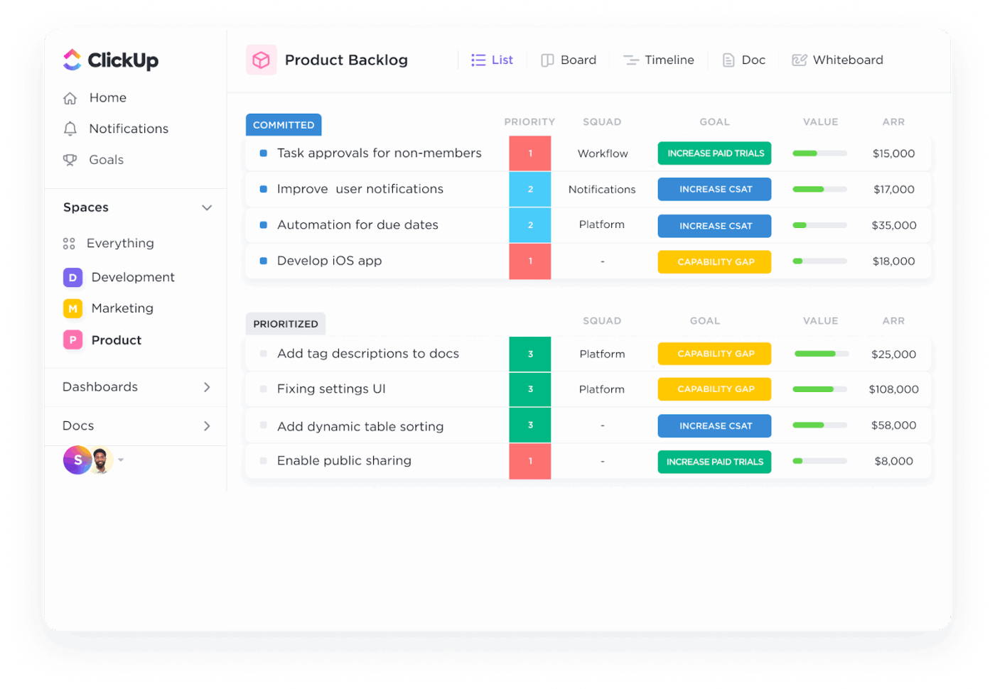
However, in the ClickUp Table View, each table-based row is a task or record, and you can sort, group, and filter your information just like Excel, but better. 

Organize your work with ClickUp

The best part? Everything stays connected. You can link a customer row to their associated invoice, delivery timeline, and support ticket without cramming complex formulas.

Here’s why the ClickUp Table View is 10x better than spreadsheet software: 

• Organize data visually by dragging and dropping columns to fit your work process
• Bulk-edit multiple entries without copying formulas or dragging cells
• Pin important columns and hide irrelevant ones to avoid feeling overwhelmed 
• Share views with internal teams or external partners through exportable and shareable tables
• Filter your table with dropdowns, tags, or Custom Fields to spotlight what matters in a few seconds

And because Table View works in sync with other views, you’re not locked into a single way of working.

ClickUp List View

The List View lets you switch from grid to checklist in seconds. Whether you’re managing a project or tracking research, it provides a clean vertical layout where each task acts like a card, complete with assignees, due dates, dependencies, comments, and attachments.

Depending on your focus, you can flip between Table and List Views: structured data or action items.

But wait, because here’s where ClickUp gets even more refreshing!

ClickUp relationships

Instead of building multiple complex spreadsheets to track relationships between people, projects, or assets, you can simply link them using ClickUp Relationships.

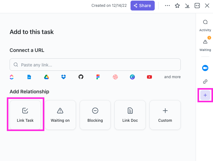
With it, you can:

• Link one task to another or Custom Fields to simulate relational data 
• Connect users to feedback, bugs to features, and deliverables to clients in one click
• Use roll-up fields to pull summary data from linked tasks, like total time spent or status updates
• Preview linked records without leaving your task screen
• Avoid broken links or mismatched references that usually plague VLOOKUP

ClickUp Custom Fields

If you need heavier datasets or data filtering, you can also try ClickUp Custom Fields.

You can create as many Custom Fields (new columns) as you want—dropdowns, dates, checkboxes, ratings, currencies, or even formulas. Just create a new field. And once your fields are in place, you can filter, group, or sort your data for your desired result.

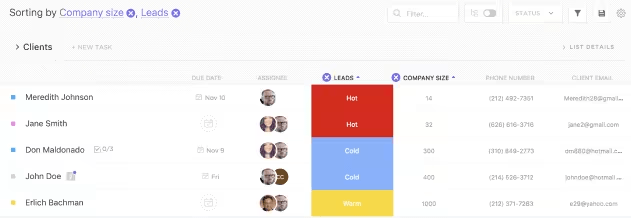
Here’s why Custom Fields is a great support:

• Add unlimited Custom Fields to tasks to capture every piece of data you need
• Filter lists and tables using Custom Field values (just like pivoting your spreadsheet)
• Group tasks by field values for clear segmentation (e.g., group leads by sales rep or region)
• Automate calculations between Custom Fields with numerical values using formula fields
• Apply the same fields across ClickUp Views to keep your data consistent, organized, and scalable

ClickUp Dashboards

After processing your data, ClickUp will also combine it using visual ClickUp Dashboards. 

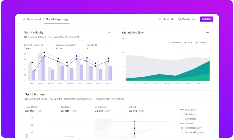
In other words, instead of exporting rows of VLOOKUP’d data to create charts elsewhere, you can build real-time dashboards with 50+ widgets here.

With ClickUp Dashboards, you can:

• Visualize data from multiple projects or departments in one place
• Build charts, bar graphs, tables, and pie widgets to represent task progress, time estimates, or revenue
• Use dashboard filters to drill down into specific Custom Fields or statuses
• Monitor each employee’s workload and capacity with the Workload View to balance your team’s resources
• Share dashboards with clients or stakeholders as live snapshots of project health

ClickUp Docs

To explain this progress to a client or stakeholder, use ClickUp Docs. 

Each document can link directly to relevant tasks, people, or assets. You and your team can also collaborate in real time on these documents to fix errors, relay information, and improve context. 

ClickUp Docs allows you to:

• Create documentation, SOPs, and reports right inside your workspace
• Embed live task lists and tables inside Docs for real-time collaboration
• Link Docs to any ClickUp Task, so context is always just a click away
• Use Docs as knowledge hubs, client portals, or meeting agendas with automatic linking

ClickUp Spreadsheet Template

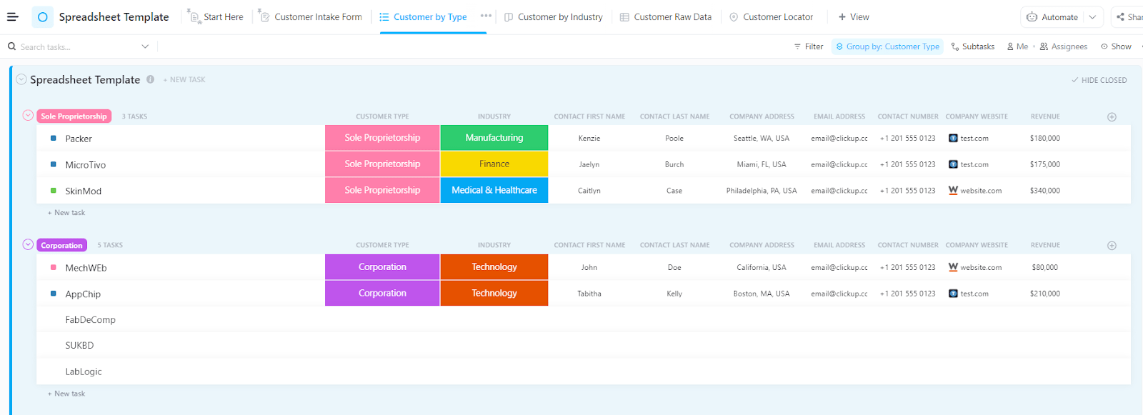
However, if you want a faster solution and something better than VLOOKUP, try the ClickUp Spreadsheet Template.

It is ideal for users who want to organize, access, and relate data without formulas. Instead of relying on static rows and columns, this template uses Custom Fields, Linked Tasks, and Table View to replicate and surpass traditional spreadsheet lookups. 

Get free template

You can create customer databases, internal tracking systems, or any workflow that needs flexible, filterable data access without formula maintenance.

With this template, you can:

• Capture important customer data using pre-formatted columns and fields
• View information in multiple formats (Table, Board, Calendar, etc.) to reduce spreadsheet complexity
• Replace VLOOKUP with linked tasks and Custom Fields to create no-code relationships between entries
• Track customer status or engagement stage using built-in statuses and filters
• Collaborate across teams by assigning owners, setting due dates, and sharing live data views in real time

Summarize this article with AI ClickUp Brain not only saves you precious time by instantly summarizing articles, it also leverages AI to connect your tasks, docs, people, and more, streamlining your workflow like never before. Summarize article

Summarize this article for me please

Want to save even more time? Try ClickUp Brain free

Ditch the Excel Formulas and Use ClickUp 

VLOOKUP serves us well, but its directionality, flexibility, and error-handling limitations have made it less suited for modern data workflows. 

Smarter alternatives like INDEX MATCH, XLOOKUP, FILTER, and QUERY offer more power, accuracy, and control over your data.

But if you’re spending too much time fixing broken formulas or managing complex spreadsheets across multiple teams, it may be time to consider a more scalable solution.

With ClickUp, you can organize and act on your data without relying on formulas. From Custom Fields to Table Views to Dashboards, ClickUp turns your data-heavy spreadsheets into a connected, visual, and collaborative workspace.

Sign up for ClickUp for free today and see how much easier data management can be!

Everything you need to stay organized and get work done.

Sign Up Contact Sales